Instantaneous Rates of Change and the Tangent Line

Need one-on-one tutoring with me? I teach all of this material! Contact me for a quick response on your needs.
Want my FULL version of these notes with more worked examples and help? Click here.

Introduction

In the previous section I introduced the concepts and math behind the average rate of change, which is the rate of change that a function would have if it were linear between the two points in the interval. However, it is a much more meaningful task to analyze how a function with curvature is changing at a moment: that is, directly surrounding a single point. This is an important issue in the history of calculus, and led to many different developments in math and capabilities in science.

The Instantaneous Rate of Change

The use of limits is fundamental in the process described above, which is why you worked on them in detail earlier in this class. To find out how to construct a rate of change for a curved function at a single point, consider the setup for finding the average rate of change, reproduced here for convenience:

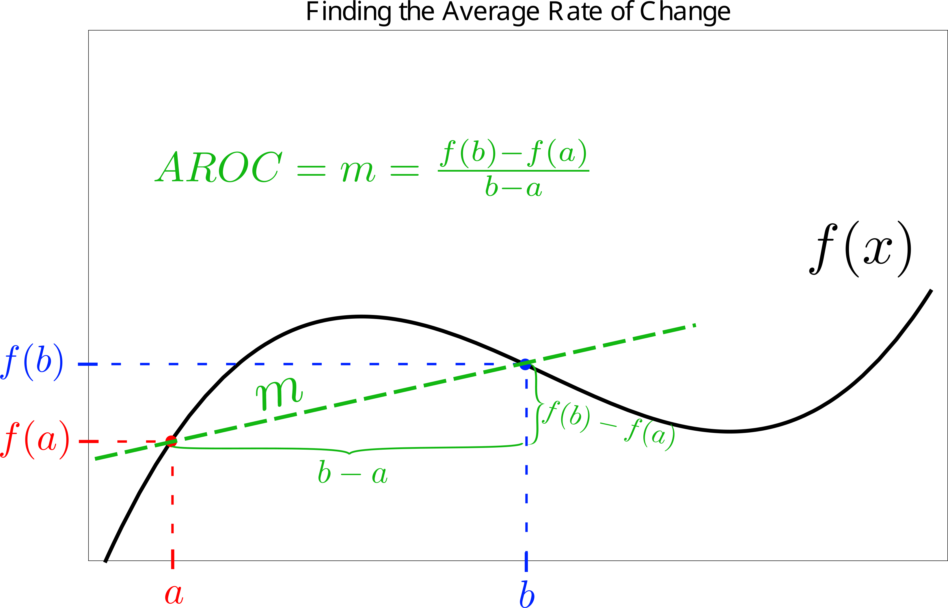This construct only gives averaged information over the interval of consideration (from $x = a$ to $x =b$ ), however. What if we’re interested in narrowing in on a specific moment to get more localized information? Well, we could simply shrink the interval of consideration down a bit more by bringing $a$ and $b$ closer together. This would begin to localize the analysis more, since the function has less opportunity to change over this smaller interval.

This process is discussed and shown, in great detail, in my full notes on this section. However, the crux of the matter is in shrinking the interval width, from $a$ to $b$ , towards zero, which makes the secant line “infinitely local”. Upon doing this, the two points come together, and we only graze the curve at one local place instead of two like before. Let’s call $a$ the leftward point in the interval and shift the rightward point toward it (to the left). We’ll call the separation distance $h$ , which makes the rightward coordinate $a+h$ . The corresponding $y$ -coordinates are then $f(a)$ and $f(a+h)$ , as shown here:

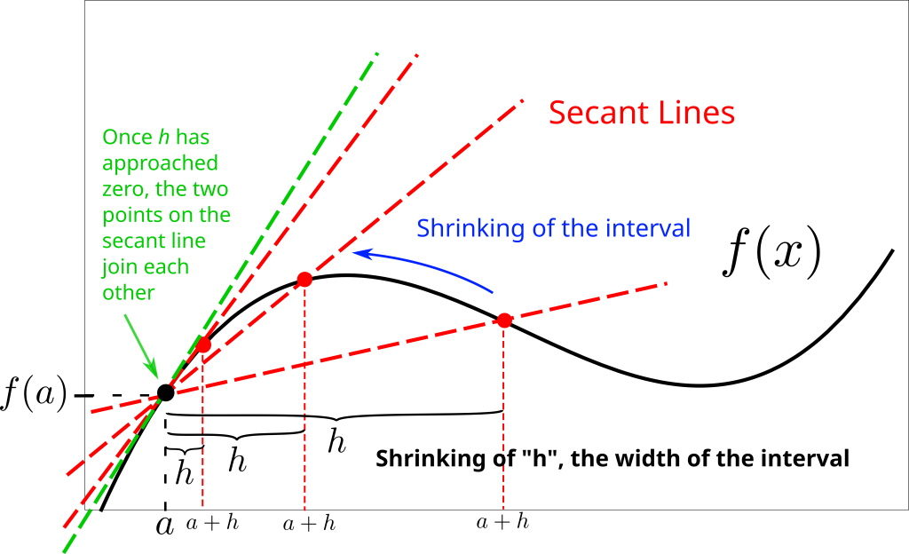
Using the average rate of change formula in conjunction with a limit as $h$ goes to zero gives us the formula for the instantaneous rate of change:

The instantaneous rate of change of a function $f(x)$ at $x = a$ is

(1) $\begin{equation*} IROC = \lim_{h \to 0} \; \frac{f(a+h) - f(a)}{h} \end{equation*}$

Now that the two points have come together (from shrinking the interval width down to zero), we are no longer dealing with a “secant” line. Instead it has a different name altogether:

A line that grazes a function at a single point locally, with slope equal to the instantaneous rate of change there, is called a tangent line.

This vocabulary makes sense because the line is “tangent” to the curve there.

The “Derivative”

The $IROC$ construction above finds the slope of the tangent line at $x$ -coordinate $a$ . However, if we use the general, unspecified value $x$ instead of $a$ , we get a function that returns the $IROC$ at any given $x$ -coordinate. This function is called the derivative of the original function, and it will be discussed in more detail next. However, it’s worth noting at this point in the material because multiple things we’ve done so far all relate to one another, and the following summary is very helpful for students:

The following are all equivalent and refer to the same quantity:

The instantaneous rate of change of $f(x)$ at $x = a$ .
The slope of the tangent line of $f(x)$ at $x = a$ .
The value of the derivative of $f(x)$ evaluated at $x = a$ .

Examples

Let’s look at some examples which will help clarify the mathematical techniques we have to use to solve the $IROC$ formula completely.

Example 1

Find the instantaneous rate of change of $f(x) =3x$ at $x = 5$ . Do it again for at $x = 8$ . What do you notice?

We use the limit of Equation 1 exactly as written in order to proceed, with $a = 5$ and $f(x)$ as given.

$IROC = \lim_{h \to 0} \frac{f(5+h) - f(5)}{h}$

where this notation is function notation (“f of five plus h” and “f of five”), and does not represent multiplication. We will end up multiplying things, however, because that’s how our function is constructed. Proceeding gives

$= \lim_{h \to 0} \frac{3(5+h) - 3(5)}{h}$

As with most limit problems, we’ll get immense help by simplifying; as it currently stands, we can’t plug in 0 for $h$ yet without getting the dreaded 0/0. Distributing the multiplication and simplifying produces

$= \lim_{h \to 0} \frac{15 +3h - 15}{h} = \lim_{h \to 0} \frac{3h}{h} = \lim_{h \to 0} 3 = 3$

where the limit in the last step doesn’t depend on $h$ , so it approaches itself as $h$ approaches zero: in this case, 3.

Try this again for $x = 8$ . What do you notice? Does this result make sense?

Example 2

Find the instantaneous rate of change of $y = -2x^2 + 3$ at $x = 1$ .

We continue working with Equation 1 to find this quantity. That looks like this:

$IROC = \lim_{h \to 0} \frac{y(1+h) - y(1)}{h}$

Plugging in gives

$= \lim_{h \to 0} \frac{[-2(1+h)^2 + 3] - [-2(1)^2 + 3]}{h}$

We now simplify the expression by expanding the term in the parentheses.

$= \lim_{h \to 0} \frac{[-2(1 + 2h + h^2) + 3] - 1}{h} = \lim_{h \to 0} \frac{2h + h^2}{h}$

We can now cancel a factor of $h$ everywhere, which eliminates the source of the indeterminate form.

$= \lim_{h \to 0} 2 + h$

$= 2$

where in the last step, I let $h$ go to 0. Therefore, the instantaneous rate of change for this parabola is 2 at $x = 1$ .

Example 3

Find the instantaneous rate of change for $g(t) = 1/t$ at $t = 5$ .

We proceed with Equation 1:

$IROC = \lim_{h \to 0} \frac{g(5+h) - g(5)}{h}$

$= \lim_{h \to 0} \frac{\frac{1}{5+h}-\frac{1}{5}}{h}$

where we now simplify this fraction with the algebra technique of your choosing. One common way is to add the fractions in the numerator by obtaining a common denominator, although I outline a more elegant method on a similar problem in my full notes on this section. Adding the fractions produces

$= \lim_{h \to 0} \frac{\frac{1}{5+h}\cdot \frac{5}{5}-\frac{1}{5} \cdot \frac{5+h}{5+h}}{h}$

$= \lim_{h \to 0} \frac{\frac{5 - (5+h)}{5(5+h)}}{h}$

$= \lim_{h \to 0} \frac{-h}{5h(5+h)} = \lim_{h \to 0} \frac{-1}{5(5+h)} = -\frac{1}{25}$

where in the last line, I had simplified the compound fraction by multiplying by the reciprocal of the denominator, and then canceled a factor of $h$ from top and bottom.

Example 4

Find the slope of the tangent line to $y = A x^2 - 4$ at $x = -3$ where $A$ is a constant.

Recall that the slope of the tangent line to a curve at a certain location is the same as the instantaneous rate of change there. We can find the slope as follows:

$m = IROC = \lim_{h \to 0} \frac{[A(-3+h)^2 - 4] - [A(-3)^2 -4]}{h}$

$= \lim_{h \to 0} \frac{A(9 - 6h + h^2) - 9A}{h}$

$= \lim_{h \to 0} \frac{-6Ah + A h^2}{h} = \lim_{h \to 0} -6A + Ah = -6A$

where the slope depends on whatever the parameter $A$ is for the parabola.

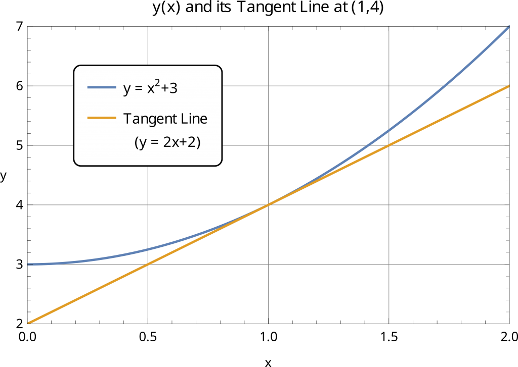
Example 5

What is the equation of the line that is tangent to $y = x^2 + 3$ at the point $(1,4)$ ?

What information do you need in order to specify the equation of a line? Consider the pieces you need in order to do so and try to find them.

There are two ways to specify a line, both of which require a slope. In addition to the slope, we need either a point on the line, or its $y$ -intercept (although these are essentially the same thing, because by knowing the $y$ -intercept, $b$ , it follows that the line goes through the point $(0,b)$ by definition.) If we can find the slope of the line, we can use this in conjunction with the given point through which it moves, and we’re done. How do we do so?

The slope of the tangent line at $(1,4)$ is the value of the instantaneous rate of change when $x = 1$ . That calculation is as follows:

$IROC = \lim_{h \to 0} \frac{[(1+h)^2 + 3] - [1^2 + 3]}{h}$

$= \lim_{h \to 0} \frac{[1 + 2h + h^2 + 3] - 1 - 3}{h}$

$= \lim_{h \to 0} 2 + h = 2$

Now we know the line has a slope of 2, and goes through the point $(1,4)$ (both the curve and its tangent line do). The equation of the line, using point-slope form, is

$y - y_1 = m(x - x_1) \Rightarrow y - 4 = 2(x - 1)$